Gamma LAT: Reference Manual

mt_lee_filt

NAME
mt_lee_filt: Multi-temporal Lee directional adaptive speckle filter

SYNOPSIS
mt_lee_filt <im_list> <ref_image> <width> <winsz> <L_ref> <L> <cthres> <out_list> [ref_out] [b_coeff] [filt_num] [msr] [ctr]

<im_list>	(input) text file with names of co-registered float format images including path (enter - for none)
<ref_image>	(input) reference image used to generate the filter weights NOTE: the reference scene should have the same dimensions as the data files in the im_list\n");
<width>	number of samples in each line
<winsz>	size of the Lee filter window (valid values: 7, 13, 19)
<L_ref>	effective number of looks (ENL) in the reference image (float)
<L>	ENL of the images in the im_list used for local determination of the the MMSE weight for each image in the im_list (float) NOTE: enter - to use the MMSE filter weight derived from the reference image for all images in the im_list
<cthres>	directional contrast threshold to determine if the directional filter should be applied (0->4)(enter - for default: 1.500) NOTE: setting cthres=0.0, forces the directional filter to be used at all times, setting cthres=4.0 blocks all directional filtering
<out_list>	list of filtered output data files, number of entries in the im_list and out_list must match, (enter - for none)
[ref_out]	(output) filtered reference image (float) (enter - for none)
[b_coeff]	(output) MMSE weighting coefficient calculated from the mean to sigma ratio and L for each sample (float) (enter - for none)
[filt_num]	(output) selected structural filter number (0-->7) (byte) (enter - for none)
[msr]	(output) mean/sigma ratio where the mean is the local mean and sigma the local standard deviation of the intensity image in the filter window (enter - for none)

Examples:

mt_lee_filt rmli_list lh_ave.rmli 600 7 100 20 1.5 rmli_lee_list lh_ave_lee.rmli lh_ave_lee.bcf lh_ave_lee.fn lh_ave_lee.msr

Filter the scenes listed in the rmli_list using filter coefficients and directional filter number derived from the averaged scene lh_ave.rmli. For each file in the input list there is a corresponding output file for the filtered data listed in the rmli_lee_list. The filtered image of the reference scene is written to the file lh_ave_lee.rmli. The filter coefficients are written to the file lh_ave_lee.bcf and the integer valued filter number (0--> 7) is written to the file lh_ave_lee.fn. The mean/sigma ratio for each point in the reference scene is written to the file lh_ave_lee.msr.

mt_lee_filt - lh_ave.rmli 600 7 100 - 1.5 lh_ave_lee.rmli lh_ave_lee.bcf lh_ave_lee.fn lh_ave_lee.msr
Same as above, but there are no files filtered, other than the reference image itself. The output files are optional.

Description

mt_lee_filt is based on an algorithm for speckle reduction described in [1] by J.S. Lee et al. This adaptive filter uses a set of 8 edge aligned window functions to select the homogeneous area associated with a particular pixel. The algorithm determines the window that best describes the region that a particular pixel belongs to. The deviation of center pixel relative to the average value over the selected window is used to determine a filter weighting factor that blends the local signal value with the average calculated using the window function. If the current pixel deviates strongly from the average of any edge aligned window function, very little or no filtering is applied. The algorithm determines both the best edge aligned filter and the weighting function. There are 8 edge aligned filters in 4 groups that are tested. The size of the window is either 7x7, 13x13 or 19x19 samples and the window functions are:

top half, bottom half
left side, right-side
upper right triangle, lower left triangle
upper left triangle, lower right triangle

The window function is either 1 or 0. Those samples where the window function is 1, are averaged in the window, while those set to 0 are ignored. The filter output is a linear combination of the local value at position x,y in the reference image and the average over the filter window. The filter has the advantage that it is effective in preserving rapid variations in backscatter, yet strongly filtering speckle noise in homogeneous regions. The user can write out the filtered reference scene, the weighting coefficient beta, the index of the selected filter window, and the mean to sigma ratio as 32-bit float computers.

The user can set a threshold for accepting the directional filtering operation based on a contrast threshold. The better the fit of the data to directional filter, the higher the contrast.
For regions with directional contrast exceeding the threshold, the directional filtering is applied, otherwise pixels from the entire region are considered. The value of the contrast varies between 0 and 4.0. If cthres is set to 0.0, then the directional filter is always applied. If the value is cthres is set to 4.0, then there will be no directional filtering.

An feature of mt_lee_filt is that the filter weight and index of the selected filter window are used to filter other scenes. Typically the reference scene used to compute the weighting coefficient and filter window is a multi-look sum and is very reliable. The other scenes are stored in a list. If there is a list of input data files, then there must be a list of the output file names provided by the user. The filter coefficients and the edge aligned filter number are then used to filter the entire stack of scenes. The user has the option to save the weighting factor, edge-aligned filter number, and the mean/sigma ratio.

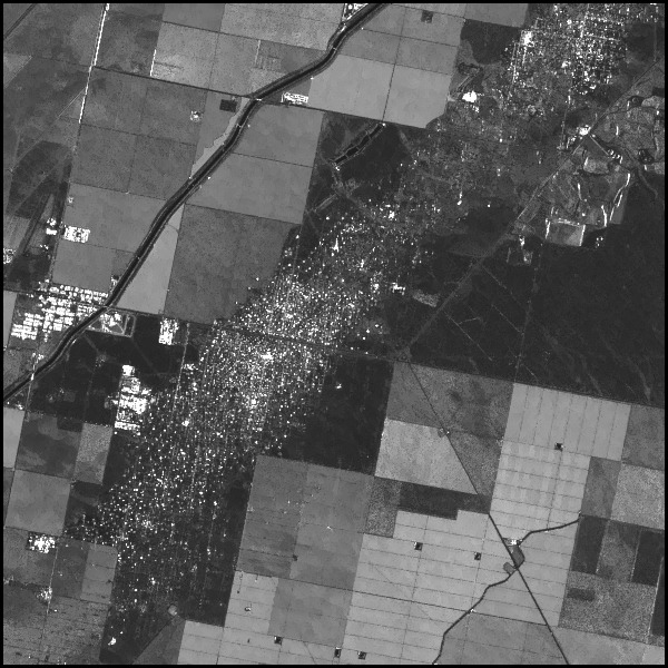
An example of a the filter in action, we use a multi-look image of the Lost-Hills oil field in California. The scene pixel sample spacing is about 15 meters in range and azimuth. The reference image is an average of 24 scenes, with each of the 24 scenes containing 5 look pixels. However the images have relatively high interferometric correlation. In this example the effective number of looks parameter L is set to 48 and the window size to 7. In the case of a homogeneous region, the number of samples in the spatial average generated by this filter is approximately 24. The original and filtered images are shown below. Note that the filter preserves resolution while filtering homogeneous regions.

Unfiltered averaged MLI image of Lost-Hills

Unfiltered reference image of Lost-Hills Oil Field. 24 images were averaged to produce this multi-look
intensity image

Filtered reference image of Lost-Hills Oil Field. 24 images were averaged to produce this multi-look
intensity image. A 7x7 filter window was used. The effective number of looks parameter L=48.

[1] Lee, J. S., S. Cloude, K. Papathanasslou, M. Grunes, I. Woodhouse, "Speckle Filtering and Coherence Estimation of Polarimetric SAR Interferometry Data for Forest Applications," IEEE Transactions Geoscience and Remote Sensing, vol. 41, no. 10, pp 2254-2263, October, 2003.
[2] Lee, J. S., Eric Pottier, "Polarimetric Radar Imaging: from Basics to Applications," Chapter 5, CRC Press, Boca Raton, 2008

SEE ALSO
temp_filt, multi_stat, mt_lee_filt_cpx